
From QAM encoding to single sideband to mixing in the optical domain — the device stays, the drive changes, Why double sideband cancels itself at some frequencies, how a 90-degree shift removes one sideband, why optical mixing needs no electronic mixer, and what folded optics is for.
On one dual-parallel Mach-Zehnder modulator, a product description usually lists three things side by side: QPSK and QAM encoding, single-sideband modulation, and RF mixing. They read as three applications. In fact they use the same electrode structure — what changes is not the device but what you drive into it.
This article takes the three apart, with the emphasis on the latter two. They are less common than data encoding, but more interesting physically, and they say more about how flexible the device is.
1. The baseline: what data encoding does
A dual-parallel structure has two Mach-Zehnder arms that can be driven independently, with 90 degrees of phase between them. Combining them gives an arbitrary point in the complex plane. That is IQ modulation: two degrees of freedom, matching the real and imaginary axes.
Feed two independent binary streams and the constellation is QPSK. Add more levels per arm and it becomes 16QAM, 64QAM. Baud rate is the number that measures it; bit rate is that times the bits carried per symbol. So "16QAM at 60 GBd" is 240 Gb per second, not 60.
The spectrum that comes out is double sideband: one copy of the modulating content either side of the carrier. For data communication that is fine — the receiver mixes the whole spectrum back to baseband with a local oscillator, and since both copies carry the same information, demodulation is unaffected.
2. Where double sideband gets into trouble
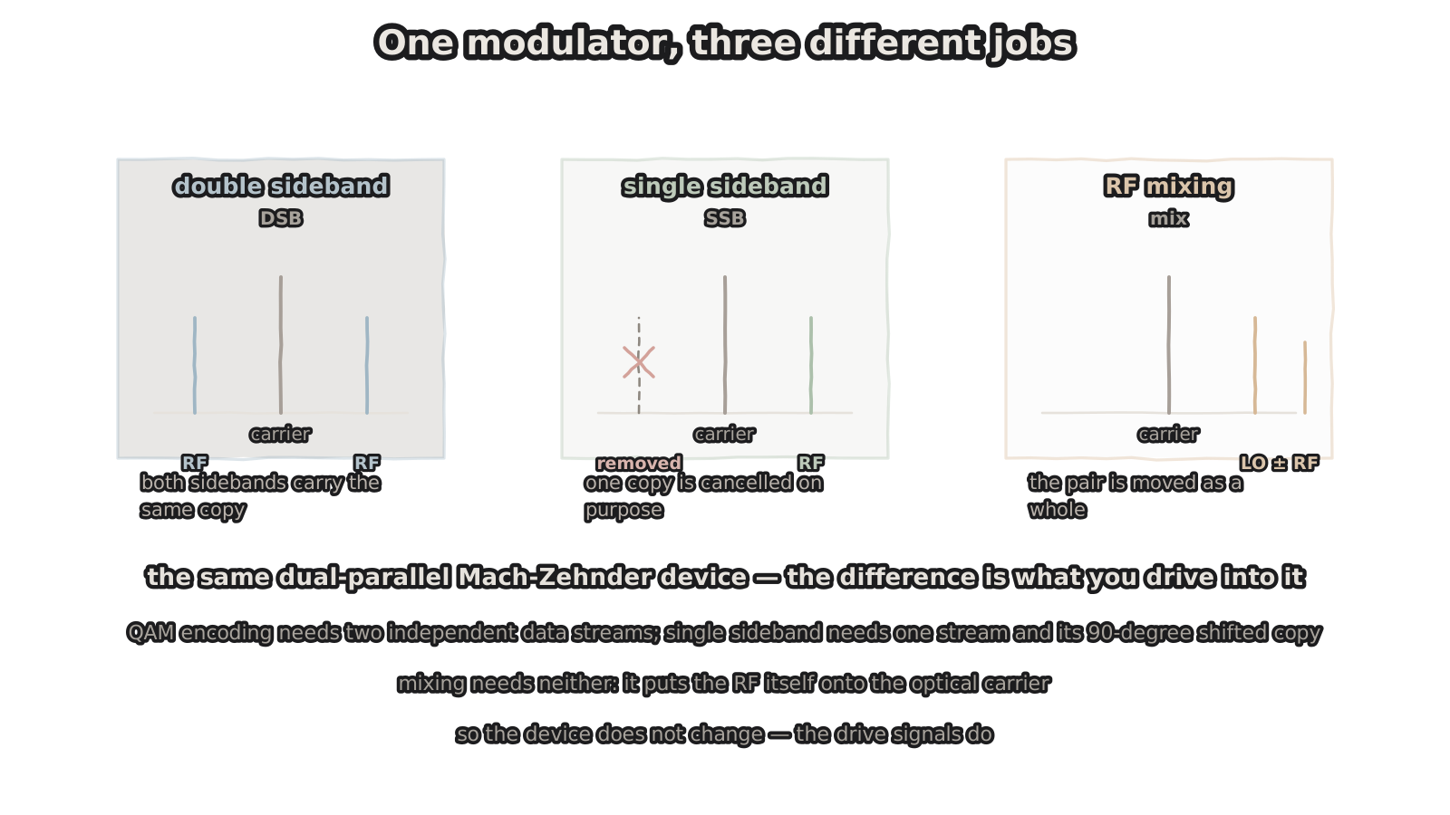
Figure 1 — One modulator, three different jobs
the device does not change — the drive signals do
Change the scenario and it breaks: radio over fibre. Here the job is not to recover digits but to deliver an analogue RF signal to the far end unchanged.
The trouble is dispersion. Refractive index varies with wavelength, so the two sidebands travel at slightly different speeds — they sit the same distance from the carrier, but one is on the long-wavelength side and one on the short.
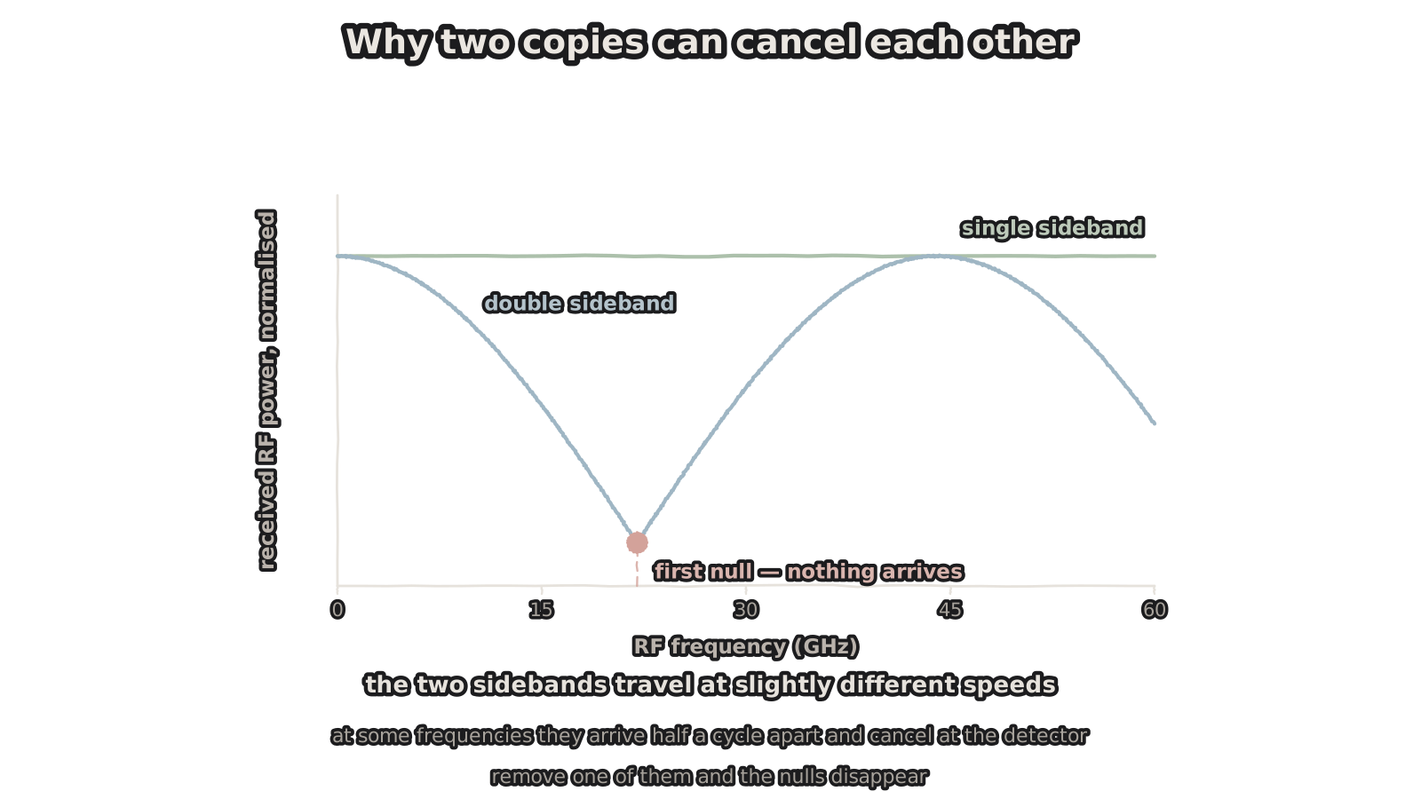
Figure 2 — Why two copies can cancel each other
at some frequencies they arrive half a cycle apart
At the detector each sideband beats with the carrier, producing two RF currents that then add. In phase, you get twice the amplitude. In antiphase, they cancel.
The phase difference grows linearly with frequency, so received power ripples with frequency as a cosine — the blue curve. At certain frequencies the power goes exactly to zero: an RF signal at that frequency simply does not arrive. It is intrinsic to double sideband, and raising transmit power does not rescue it, because the signal vanishes along with its own copy.
Worse, where the first null falls is set by fibre length and dispersion coefficient. Change the link and the nulls move.
3. Single sideband: remove one copy
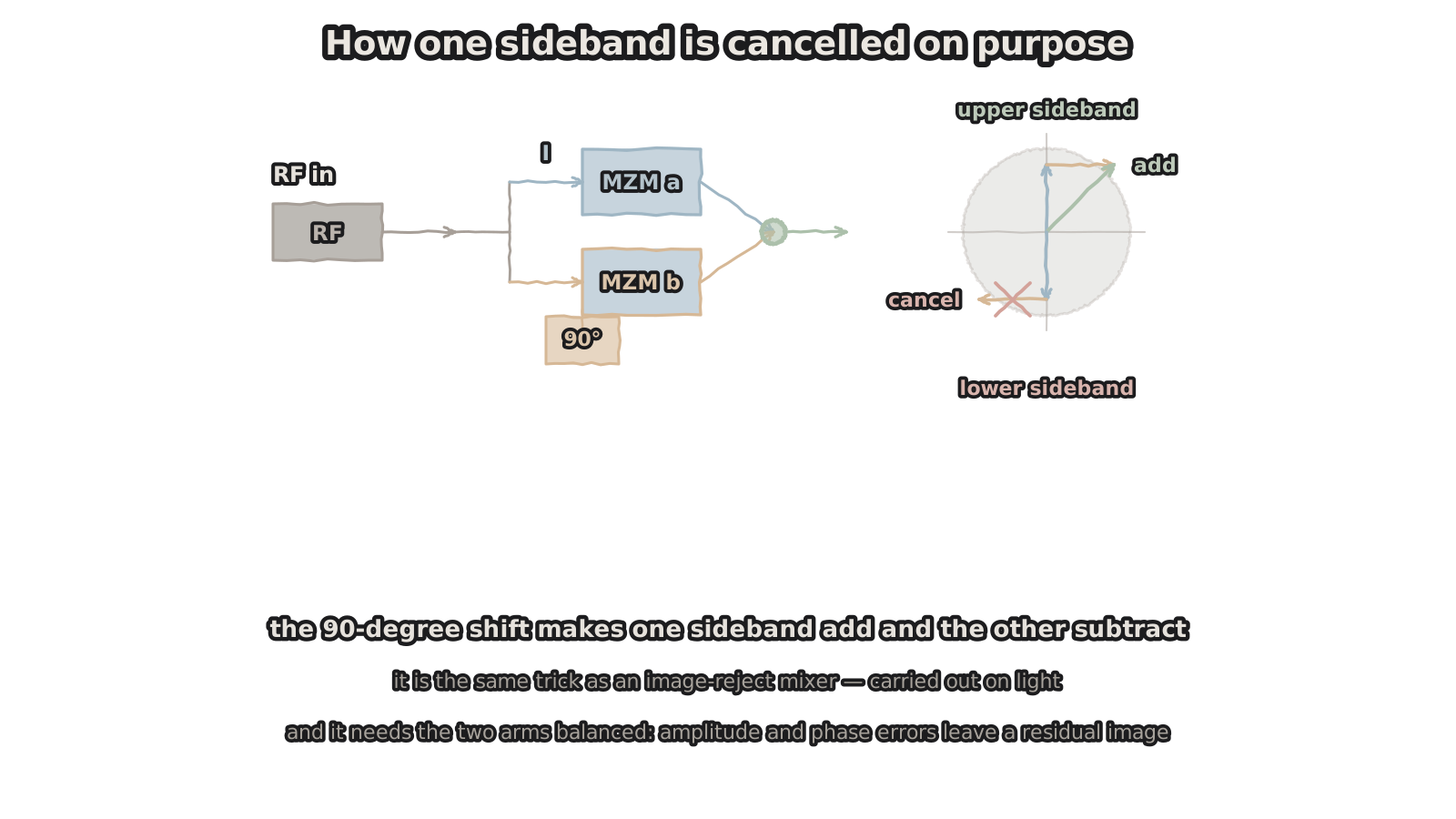
Figure 3 — How one sideband is cancelled on purpose
the 90-degree shift makes one add and the other subtract
If two copies are the problem, drop one. That is single sideband.
The implementation is neat, and it uses the same IQ modulator: split the RF signal in two, shift one branch by 90 degrees, and feed the two into the I and Q arms.
Seen in the complex plane: the two contributions at the upper sideband are in phase and add; at the lower sideband they are in antiphase and cancel. What remains is a single sideband.
This is single-sideband modulation, which is also an image-reject mixer carried out on light — the classic RF technique for suppressing an unwanted sideband, moved into the optical domain.
The cost is that it demands good balance: unequal amplitudes, or a phase shift that is not exactly 90 degrees, and a residual image sideband stays behind. Practically, 20 to 30 dB of suppression is achievable, and every dB beyond that is hard. Which is also exactly what the same device needs in QAM mode — balanced arms are a precondition for IQ modulation anyway.
Remove one sideband and the nulls in Figure 2 disappear. With one copy left there is nothing for it to cancel against. That is the flat green line.
4. Mixing: no data needed at all
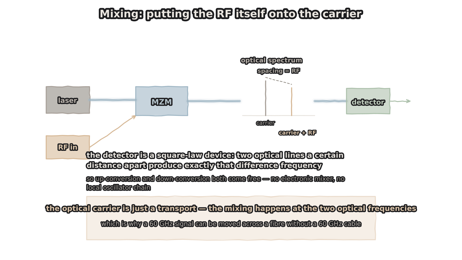
Figure 4 — Mixing: putting the RF itself onto the carrier
the detector is square-law: the spacing is the difference frequency
The third connection is more direct: send no data — put the RF itself onto the optical carrier.
Bias the modulator at a chosen point on its transfer curve and apply the RF straight to the electrodes. The output spectrum contains the carrier and components at carrier plus and minus the RF frequency — two lines separated by exactly the RF frequency.
Then land that light on a detector. A detector is a square-law device: output current is proportional to the square of the optical field, so the two lines beat and what comes out is their difference frequency — the original RF.
What makes this worth doing: neither up-conversion nor down-conversion needs an electronic mixer, nor a local-oscillator chain. The translation happens in the optical domain; the fibre just transports.
So put a detector at the far end and a 60 GHz signal appears at its output — the path in between is fibre, not 60 GHz coax. Back to the comparison in an earlier article: coax loss rises with frequency, fibre loss does not. That is precisely the property this connection exploits.
Phase noise benefits too. In the electronic route, multiplying a low-frequency signal up to millimetre waves degrades phase noise by 6 dB per doubling; with optical beating, phase noise depends only on the linewidths of the two lasers and not at all on multiplication factor.
5. At 60 GHz, the package matters more than the chip
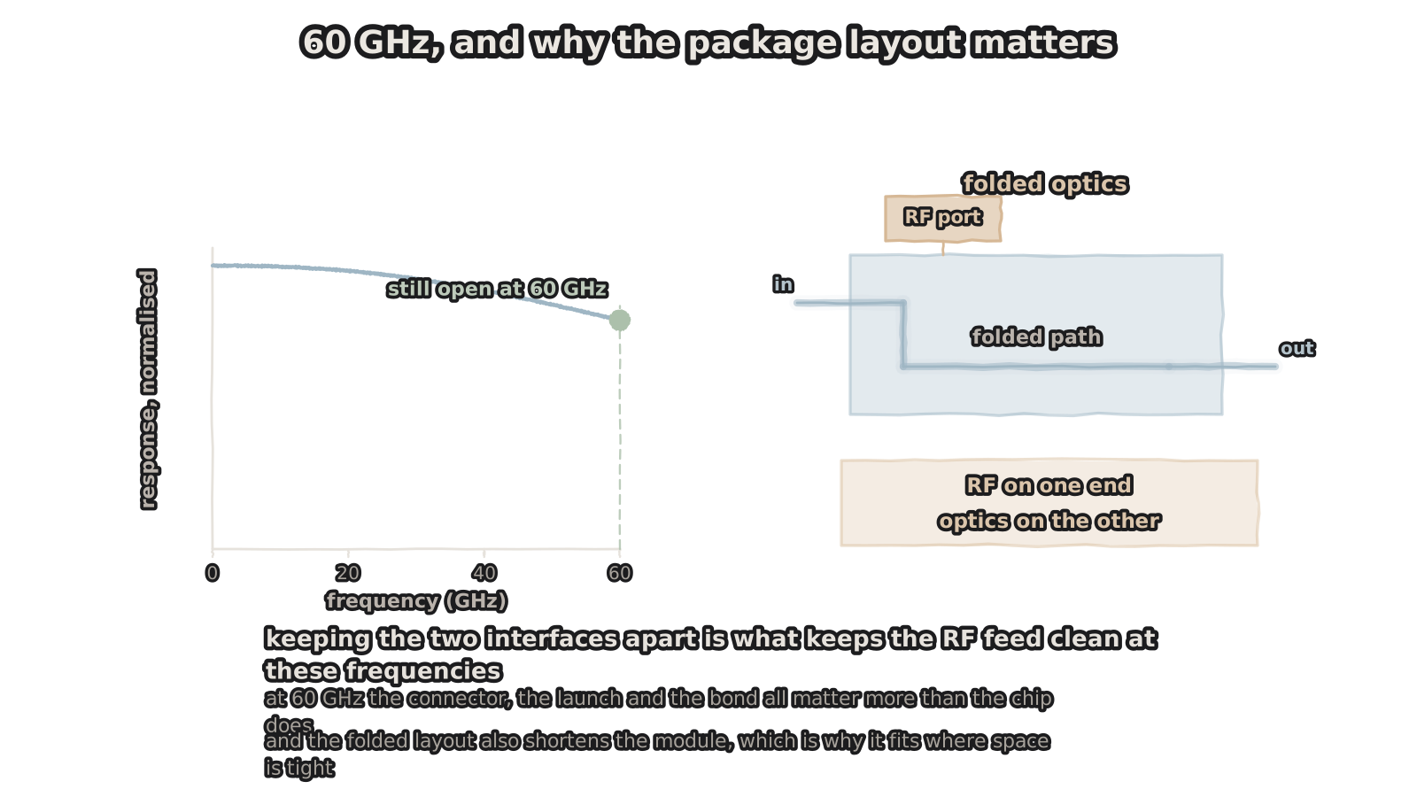
Figure 5 — 60 GHz, and why the package layout matters
RF on one end, optics on the other — it matters at 60 GHz
All three connections run at frequencies in the 60 GHz region, and at that point what decides the outcome is usually packaging rather than the chip.
The RF arrives through a connector and reaches the electrodes through bonds, and any discontinuity along that path reflects. At 60 GHz the connector, the launch and the bond matter more than the die does — a chip that runs to 110 GHz does not guarantee the packaged module still does.
That is what folded optics is for: the RF interface sits at one end of the device and the optical interface at the other, physically apart. The RF feed is not interrupted by the optical coupling structures, so its integrity is preserved; and folding the optical path into a U shortens the module, which matters where space is tight — airborne, spaceborne.
The response curve in Figure 5 makes a separate point: leave margin on the chip bandwidth. With the signal at 60 GHz, the response is still open there, which says the design has headroom. Specify right at the 3 dB point and the extra loss the package adds eats it directly.
6. What to ask
If these modes are what you need, these are the items worth pinning down.
Sideband suppression — measured in SSB mode, 20 dB or 30 dB, and whether there is a curve against frequency. Amplitude and phase balance between the two arms — it sets both the error vector magnitude in QAM and the suppression in SSB. Bias point and linearity in mixing mode — where it is biased, and what input RF power starts to compress it. RF connector type and rating — 2.92 mm series or higher, and how far above the signal frequency. Package form — folded optics or not, RF and optics at opposite ends or not. The response curve, not a single number — the whole S21, to see what margin is left at 60 GHz.
That last one is the easiest to skip. A datasheet gives "60 GHz bandwidth" as a figure, but what is useful is how much of the curve is left at the frequency you intend to use. Meeting the number and meeting the curve are different things.
Closing
One dual-parallel modulator: two independent data streams and it does QAM; one signal plus its 90-degree copy and it does single sideband; apply the RF directly and it mixes.
All three share the same physical structure. Only the drive differs. That property — one device covering several functions — says more about the value of an integrated photonics platform than any single specification does. It is not a part customised for one application; it is a primitive that can be configured again and again.
The device stays and the drive changes. Data encoding needs two degrees of freedom, single sideband needs one signal and its 90-degree copy, and mixing needs no data at all — the RF is the signal.
Figures are hand-drawn vector schematics illustrating structure and principle; they do not represent the actual shape, dimensions or layout of any specific product.
Baud rates, frequencies, sideband suppression and response figures quoted are illustrative or typical values for volume parts; actual numbers depend on device design, package form and operating conditions.