
Balanced detection needs two matched paths, and matching is not one number, Why coherent reception needs two detectors, how mismatch eats common-mode rejection, saturation at high power, and why the two ends of 780–2500 nm are not equally hard.
On a high-speed photodetector datasheet the most prominent number is bandwidth — 110 GHz. It matters, but it describes a single device. The coherent receiver that actually uses it needs two, and those two have to be a pair.
This article is about pairing: what has to match, what happens when it does not, and why buying two identical detectors is not the same as buying a pair.
1. Why two, not one
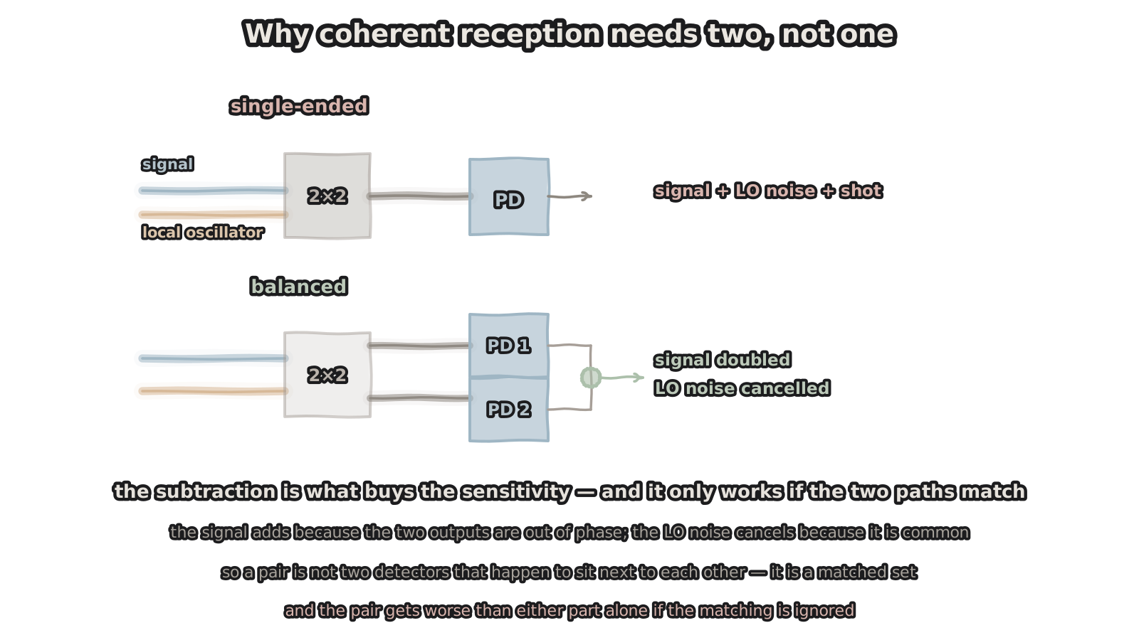
Figure 1 — Why coherent reception needs two, not one
the signal adds; the LO noise cancels
A coherent receiver sends the signal and the local oscillator into a 2×2 coupler and gets two outputs. Those outputs have one crucial property: the signal components are out of phase, the LO components are in phase.
With one detector you can only take one output. You get the signal, plus all of the LO noise — and the relative intensity noise of a local oscillator is usually well above the shot noise of the signal itself, so it sets the sensitivity.
With two, each takes one output and the currents are subtracted. The result: the signal adds, because it was out of phase, doubling the amplitude; the LO noise cancels, because it was common. That is where the sensitivity gain of balanced detection comes from.
The catch is that subtraction only works when the two paths are symmetric. So a pair is not two devices that happen to sit next to each other — it is a matched set. And when matching is ignored, the combination performs worse than either device would alone.
2. What mismatch costs
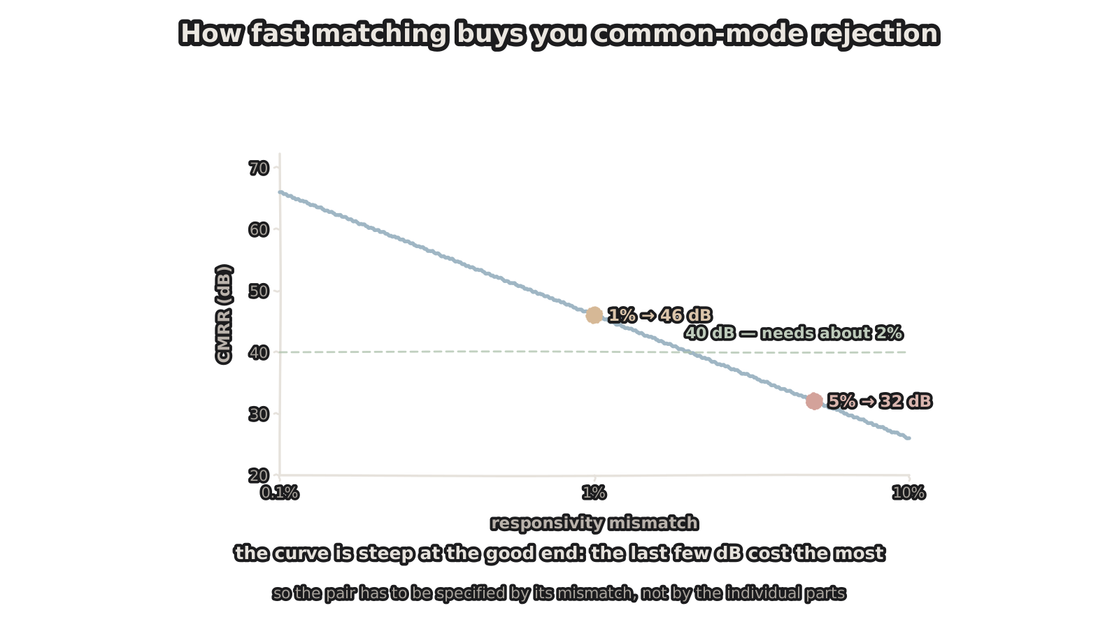
Figure 2 — How fast matching buys common-mode rejection
steepest at the good end — the last few dB cost the most
The consequence can be quantified. With responsivities R₁ and R₂, the common-mode rejection ratio is the sum over the difference:
CMRR = 20·log₁₀[ (R₁ + R₂) / (R₁ − R₂) ]
A few numbers make it concrete: 1% mismatch gives 46 dB, 5% drops to 32 dB, and 10% leaves only 26 dB. Read the other way, 40 dB of rejection requires the responsivity mismatch to be held inside 2%.
One feature of that curve is worth noting: it is steepest at the good end. Improving from 10% to 5% recovers 6 dB; improving from 2% to 1% also recovers 6 dB — but the second is far harder to make. The last few decibels are the most expensive.
So the right way to specify is not "two 110 GHz detectors" but "a pair, with mismatch below some value". The first constrains the individual part; the second constrains the combination.
3. Four things have to match
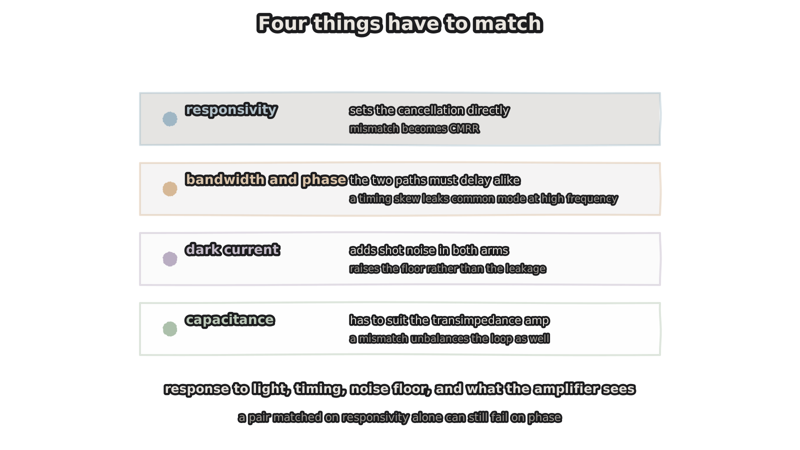
Figure 3 — Four things have to match
matched on responsivity alone, it can still fail on phase
Responsivity is only the first. Four items, taken together.
Responsivity — sets the cancellation directly; it is the horizontal axis of the curve above.
Bandwidth and phase — the two paths have to delay alike. This one is easy to miss, because datasheets usually give bandwidth, which is an amplitude response, while it is the phase response that tells you whether the two paths are synchronous. A phase difference at high frequency lets common-mode content leak through at particular frequencies, showing up as a noise floor that ripples with frequency.
Dark current — contributes shot noise in both arms. It raises the floor rather than the leakage. Note that its consequence differs from responsivity mismatch: one lifts the noise floor, the other lets LO noise in.
Capacitance — has to suit the transimpedance amplifier that follows. If the two differ, it does not merely affect the two frequency responses; it unbalances the amplifier loop itself.
In one line: a pair matched on responsivity alone can still fail on phase.
4. The other axis: power
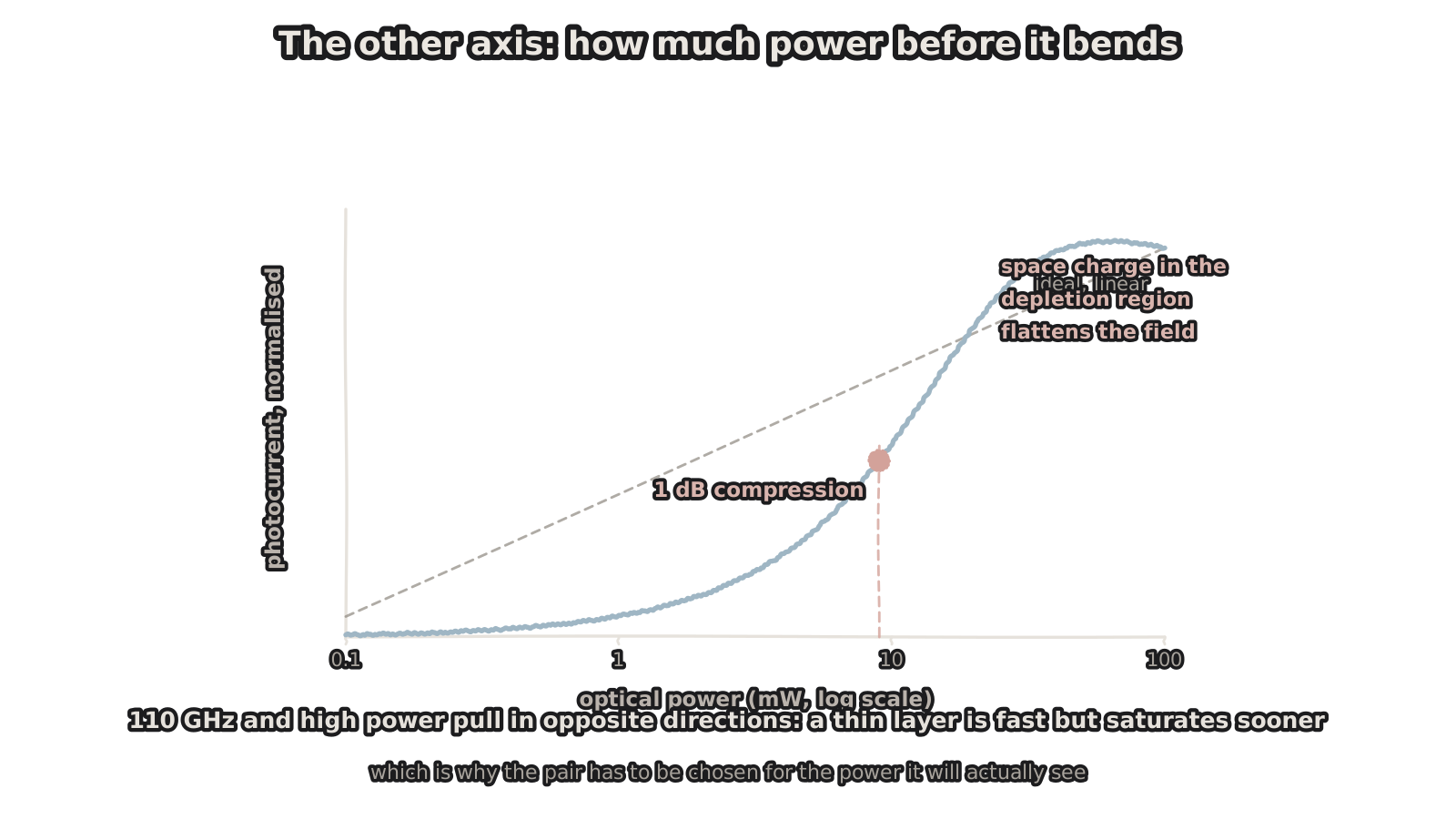
Figure 4 — The other axis: how much power before it bends
110 GHz and high power pull opposite ways: thin is fast but saturates sooner
Beyond pairing there is another axis that is often skipped: how much light this detector will actually see.
Ideally photocurrent is proportional to incident power. Push the power up and the curve bends — photo-generated carriers accumulate in the depletion region, screening the internal field, and collection efficiency falls. The bend is marked in practice by the 1 dB compression point.
The trouble is that bandwidth and power pull in opposite directions. To be fast, the absorption layer has to be thin: short transit time, small capacitance. But a thin layer also has small volume, so space charge sets in earlier at a given power density and the saturation point drops. "110 GHz" and "high power" are competing demands on the same device.
That bears directly on selection: choose for the power you will actually apply, not the largest number on the datasheet. A coherent receiver running a strong local oscillator and a sensing application working with a faint signal want different device designs.
5. 780 to 2500 nm: the ends are not equally hard
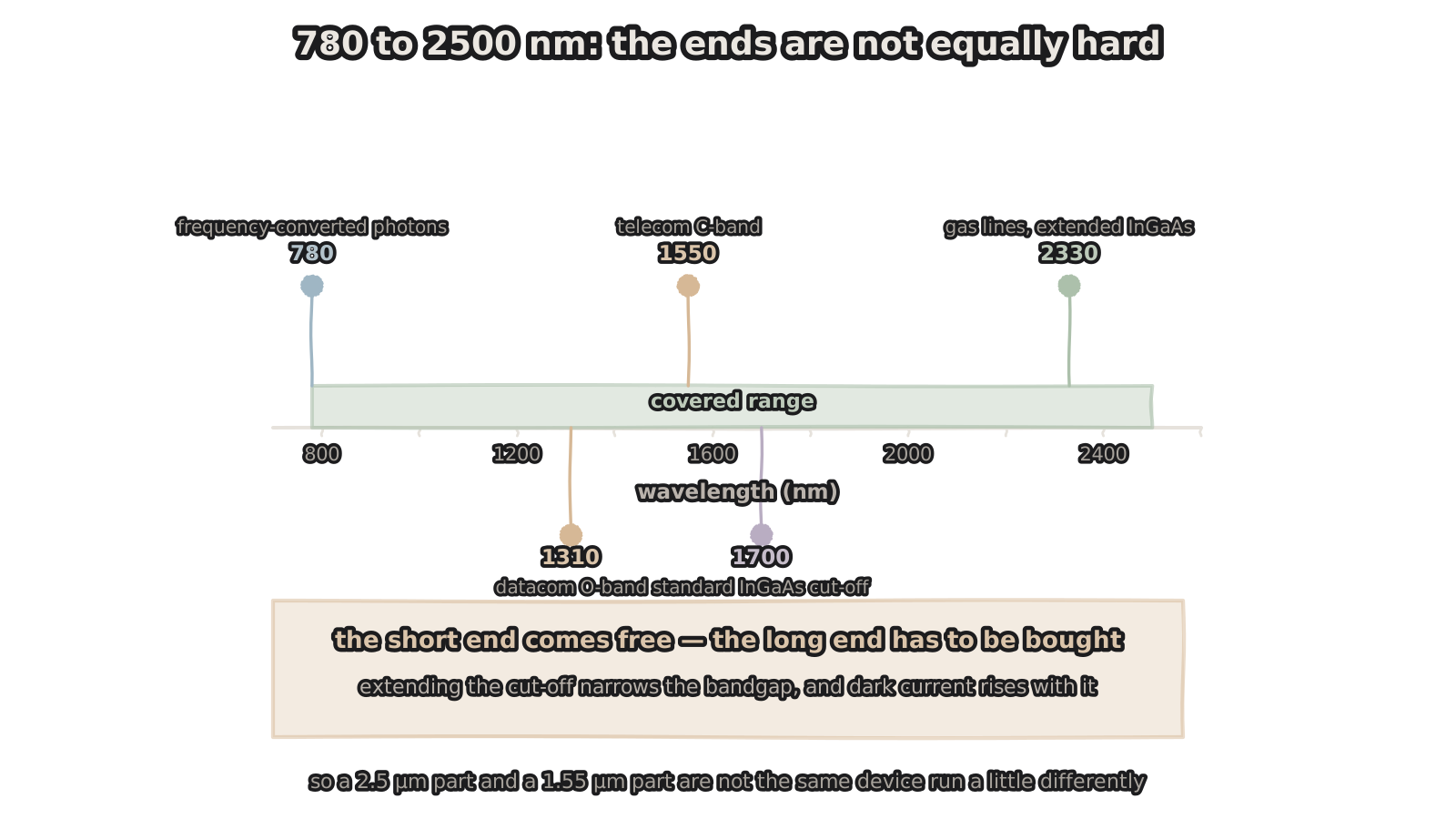
Figure 5 — 780 to 2500 nm: the ends are not equally hard
the short end comes free; the long end costs dark current
Last, the wavelength coverage. A specification reading "780 to 2500 nm" looks like a uniform range. The two ends are nothing alike in difficulty.
Mark the familiar points on that axis: 1310 nm is the datacom O-band, 1550 nm the telecom C-band, and both are routine operating points for volume parts; out near 1700 nm sits the cut-off of standard InGaAs; and the gas absorption lines beyond 2000 nm are only reachable with an extended cut-off.
The short end comes free. InGaAs has its absorption edge near 1.7 µm, so everything shorter is absorbed — 780 nm falls inside the range without any additional work. What matters at that end is on the application side: it is where a frequency-conversion module lands communication-band photons, and it is where silicon detectors work best.
The long end has to be bought. Standard InGaAs cuts off at 1.7 µm. Pulling the cut-off out to 2.5 µm means raising the indium fraction and narrowing the bandgap — and as the bandgap narrows, thermally generated carriers rise exponentially, dark current follows, and stronger cooling is usually needed to hold it down.
So a 1.55 µm part and a 2.5 µm part are not one device run with different settings. They are different material designs. Specify for the wavelength you actually use rather than paying in dark current for coverage you do not need.
6. What to ask
Pulling it together, these are the items worth pinning down when specifying or accepting delivery.
Single or paired — for balanced detection you need a pair. The mismatch figure — the upper bound on responsivity mismatch, and whether there is any phase or delay consistency data. Common-mode rejection — measured, and as a curve against frequency rather than a single number. What the bandwidth means — 3 dB electrical or optical, and under what test conditions. 1 dB compression and saturation power — checked against your actual LO power. Dark current and capacitance — the first sets the noise floor, the second decides how well it matches the amplifier. Wavelength version — standard or extended cut-off, and how much dark current differs between them.
One more worth raising unprompted: can the pairing be screened to the application conditions. If the two key parameters can be measured at wafer level, matching by lot is more reliable — and cheaper — than selecting afterwards.
Closing
110 GHz says how fast one detector can run. What the receiver actually needs is two detectors that run at the same speed.
Those are not problems of the same order. The first is solved by device design; the second by design and screening together — and screening only becomes practical on a platform that runs at volume and can measure in batches.
Bandwidth is a property of one device; pairing is a property of the combination. Coherent reception buys the second, and the second is exactly the half that datasheets most often leave out.
Figures are hand-drawn vector schematics illustrating structure and principle; they do not represent the actual shape, dimensions or layout of any specific product.
Bandwidth, common-mode rejection, compression point, dark current and other figures quoted are illustrative or typical values for volume parts; actual numbers depend on device design, process platform and pairing scheme.